Google Sheets IF functions offer the ultimate spreadsheet solution when you want to include condition-based formulas that act like interactive flow charts. By evaluating specific criteria at each juncture, these functions allow your data to return specialized results based on whether conditions evaluate to true or false.
Google Sheets IF functions crafted with logical capabilities—from basic comparisons and multi-criteria evaluations to specialized conditional averages, sums, counts, and error handlers—transform how you build responsive and robust spreadsheet tools.
IF
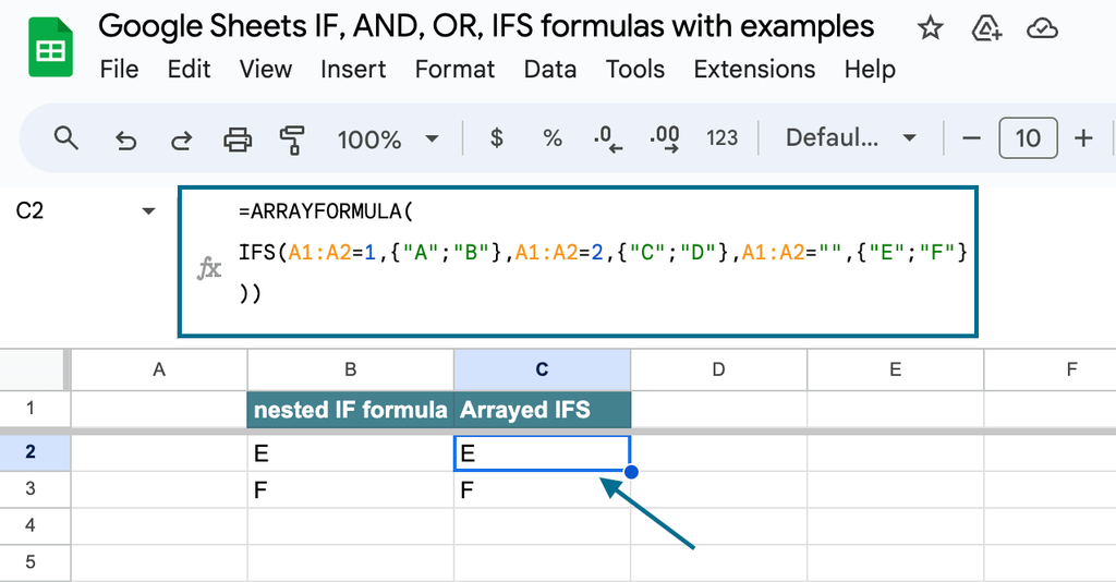
This is the most basic function in this category. Basically, it evaluates a single condition and outputs different results if it’s TRUE or FALSE.
=IF(condition, value_if_true, value_if_false)
IF is great to make simple logical comparisons. For example, you can evaluate whether students “Pass” a test if their score is over 50.
Note: given the formula below students who got exactly 50 will also be assigned a “Fail”.
=IF(A1 > 50, “Pass”, “Fail”)
IFS
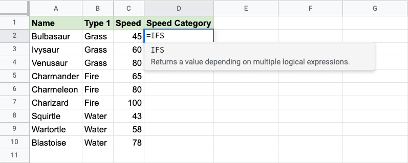
This function has a number of conditions and values. The first condition to be TRUE will return its corresponding value.
=IFS(condition1, value1, condition2, value2, …)
The IFS function is useful to evaluate multiple conditions against a set of values. For example, we could use it to translate grades from percentages to letters.
=IFS(A1 > 90, “A”, A1 > 80, “B”, A1 > 70, “C”, A1 > 60, “D”, TRUE, “F”)
AVERAGEIF
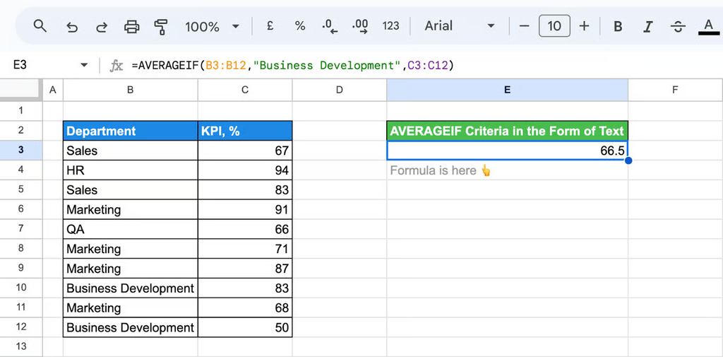
Calculates the average of a range of cells that meet a specified condition.
=AVERAGEIF(range, criterion, [average_range])
The AVERAGEIF function is useful to limit the values you want to average. Continuing with the test example, we could use it to find the average test score for students who passed.
=AVERAGEIF(A1:A10, “> 50”)
AVERAGEIFS
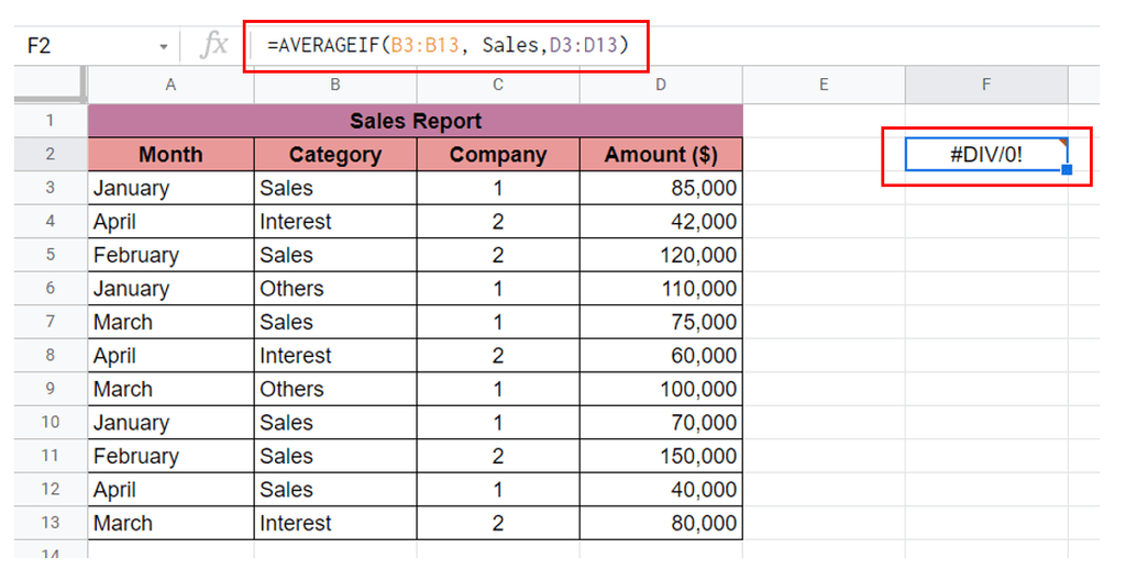
Calculates the average of a range of cells that meet multiple specified conditions.
=AVERAGEIFS(average_range, criteria_range1, criterion1, criteria_range2, criterion2, …)
AVERAGEIFS lets you set multiple conditions to narrow down the values to include in your average. For example, you could average the test scores for students who passed and are right handed.
=AVERAGEIFS(B1:B10, A1:A10, “Pass”, C1:C10, “Right”)
COUNTIF
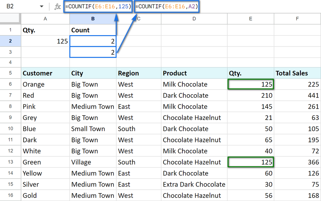
Counts the number of cells in a range that meet a specified condition.
=COUNTIF(range, criterion)
This function is great to know how many students passed the test.
=COUNTIF(A1:A10, “>50”)
COUNTIFS
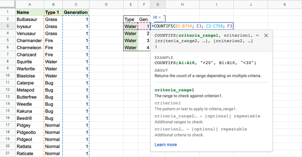
Counts the number of cells in a range that meet multiple specified conditions.
=COUNTIFS(criteria_range1, criterion1, criteria_range2, criterion2, …)
Again, say you are fixated on your right handed students. COUNTIFS will let you know how many of them passed the test.
=COUNTIFS(B55:B65, “> 50”, C55:C65, “Right”)
SUMIF
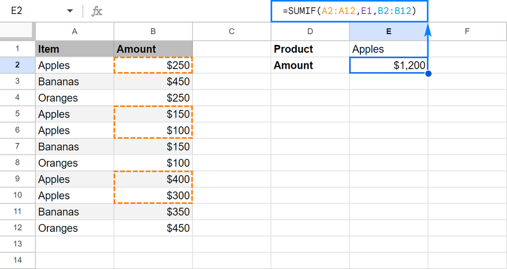
Adds certain values based on a single condition.
=SUMIF(range, criterion, [sum_range])
The SUMIF function is useful to single out certain values you want to add. It can calculate total sales for a product, sum expenses for a category, or add scores above a threshold.
=SUMIF(A1:A10, “Product A”, B1:B10)
SUMIFS
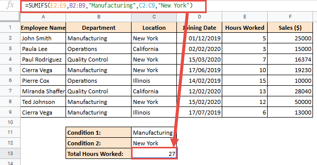
Adds the cells in a range that meet multiple conditions.
=SUMIFS(sum_range, criteria_range1, criterion1, criteria_range2, criterion2, …)
The SUMIFS function is perfect for adding up values that meet multiple criteria, such as summing sales only for a specific region and product.
=SUMIFS(B1:B10, A1:A10, “North”, C1:C10, “Product A”)
SWITCH
Tests an expression against a list of cases and returns the corresponding value of the first match. It’s a great alternative to nested IF statements because of its increased simplicity and readability.
=SWITCH(expression, case1, value1, case2, value2, …, [default])
The SWITCH function is useful when you have multiple conditions to evaluate and want to return a specific value for the first true condition.
=SWITCH(A1, “Red”, 1, “Green”, 2, “Blue”, 3, “Unknown”)
IFERROR
Returns a value if there is no error, otherwise it returns a specified value if there is an error.
=IFERROR(value, [value_if_error])
The IFERROR function is useful to handle errors in formulas. It helps ensure that your spreadsheet doesn’t show errors and displays user-friendly messages instead.
=IFERROR(100/0, “Divide by zero error”)
IFNA
Returns a specified value if the formula evaluates to #N/A; otherwise, it returns the result of the formula.
=IFNA(value, value_if_na)
The IFNA function is great for handling the #N/A error specifically, ensuring that your spreadsheet can display a custom message or alternative value when this error occurs.
=IFNA(VLOOKUP(A1, B1:B10, 2, FALSE), “Not Found”)
Conclusion
Google Sheets’ IF functions allow you to include condition-based formulas in your spreadsheets. They act like flow charts that guide your data processing based on specific conditions.
From the basic IF function to more advanced ones like IFS, SUMIFS, and SWITCH, these functions perform complex logical operations.